It’s been a while and the teams are already deep into the Bundesliga season. Nevertheless, I don’t want to deprive you of my findings of simulating the strategy. In the first post, we looked at 14 seasons of Bundesliga data to analyze patterns in match results, goal times and odds trends.
Our Strategy
The strategy I will be backtesting today will be betting on over 0.5 goals in the 30th minute if until then no goal has been scored. At the time of writing the odds with these conditions average at around 1.2. The odds are crucial to the profitability of this strategy, so keep that in mind. I will walk you through my analysis and thoughts when writing the code for it. You can download the unfortunately unorganized notebook and the data for this study.
For the following study, I used a technique called hyperparameter optimization, which is a common method in Machine Learning to systematically adjust the parameters of a model to improve its performance on a specific task, such as enhancing accuracy, reducing error rates, or optimizing computational efficiency. In my case, I tried to optimize the following parameters to achieve the highest chance of being profitable with my betting strategy:
- x: margin per bet in percent (1-100%)
- y: max win series before securing profits (1-20)
- z: cashout after y winning bets (1-100%)
Essentially I wanted to see with how much margin x I should bet and after how many winning bets y I should cash out z percent. The idea is that you start with let’s say 100$ initial investments with x=10%, y=5, and z=50%. I would start with 10$ on the first bet. If won I would keep betting with the money I made from the first bet. So if the odds had been 1.16 when I entered the bet, I would now bet with 11.6$ on the second bet. Let’s say I win 5 (y) bets in a row, assuming the odds are 1.16 on all bets I would have 90$ on my account + 20.1$ in my bet. After the winning streak of 5 bets. I would cash out 50% of the 20.1$ to my account balance, bringing me to 100.05$ on my account and 10.05$ left for the sixth bet.
You might ask why I didn’t optimize for a simple x% margin per bet, like 10% on every bet for example. As this strategy will have lots of winning bets, as the odds are very small (~1.16), I wanted to have an additional compounding effect in it. I am aware that this adds additional risk, but potentially higher returns in the long run. Additionally, the simple approach has been neutralized by the betting service with a higher probability than my more complex approach. In the end, we have to keep in mind that we essentially try to find a hole in the betting services’s calculations, which is not easy and possibly not manageable to do so.
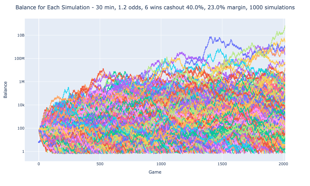
Going back to my parameter optimization. By running all 210.000 combinations of the params I found out that the best settings are the following: x = 23%, y = 6, z = 40%. The following graphs will now always use these settings to perform the simulations of my strategy.
Simulation Results
Balance Over Time for Each Simulation

This graph shows the balance trajectory for individual simulations. Each line represents one of 1000 simulations of betting on matches with specific odds. The y-axis depicts the balance, and the x-axis tracks the progression of bets placed. The wild fluctuations in the beginning reflect how randomness significantly impacts short-term results. However, some trajectories stabilize over time, revealing the potential for consistent profitability under the right conditions.
Distribution of Bets Before Losing All Money

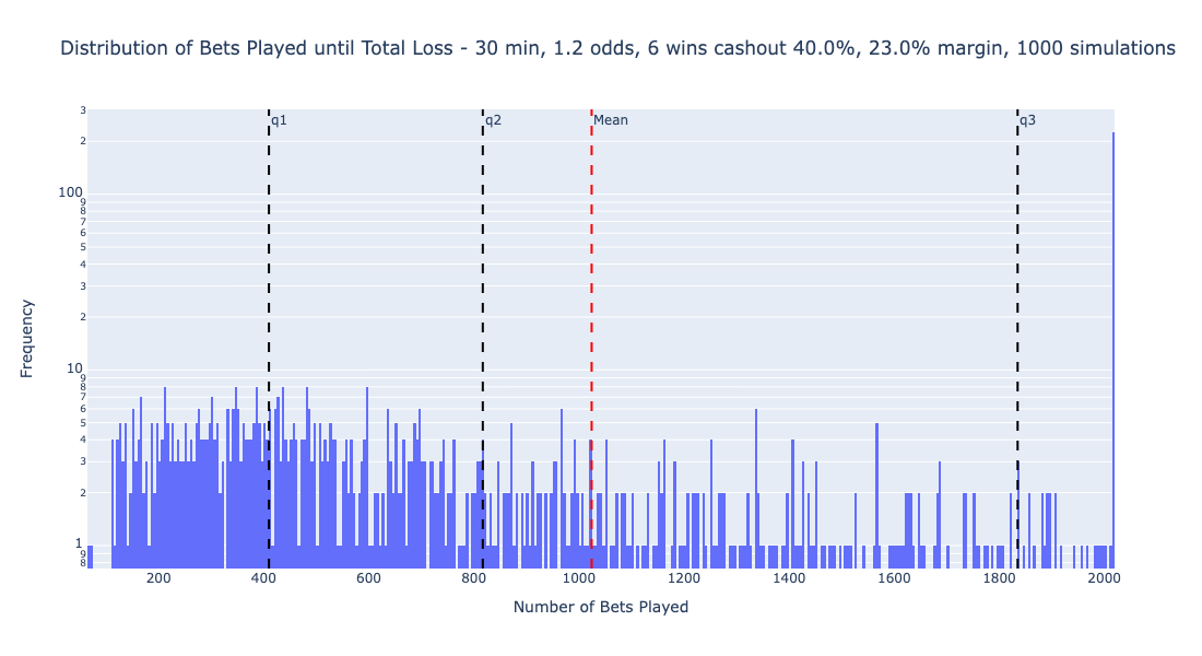
The histogram shows most simulations end quickly, as seen in the high density on the left side. Outliers skew the mean (red line), indicating in some simulations the money lasts significantly longer than average. The quartiles (q1, q2, q3) provide a clearer representation of typical performance, with the second quartile (q2) aligning closer to the majority’s outcomes. This emphasizes the median as a better indicator of the typical bettor’s experience over the mean. However we also see that about 20% of the simulations pass the 2000 bets and never suffer a total loss. A further interesting exploration would be checking how many bets are placed on average per season to make that chart more accessible.
Median Simulation Results

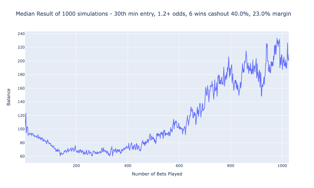
This plot depicts the balance progression for the median simulation result. The strategy leads to losses early on, but after about 150 bets, the balance stabilizes. The eventual upward trend indicates a potential recovery phase, though the risk of bankroll depletion remains significant. The mean result differs significantly from the median. A small subset of simulations performed exceptionally well as seen in the first graph, skewing the mean and suggesting having found a really great strategy. It’s a good reminder to assess both mean and median performance metrics when evaluating a strategy.
Conclusion
It seems like this strategy can be sort of profitable as seen in the last graph. Nevertheless, we have seen the huge variations of the simulations, so in the end, it seems to be a gamble. You might call it “roulette with a minimal higher chance of winning”. Also note that we have chosen the best parameters in the backtest, so we may have fallen victim to the hindsight effect. I hope you enjoyed this study!
All graphics were created by me using Python and are available for non-commercial use. Please note that the analysis and calculations presented here may contain errors.